How To Give A Large Data Into Numpy Arrays

Broadcasting¶

The term dissemination describes how NumPy treats arrays with dissimilar shapes during arithmetic operations. Subject area to certain constraints, the smaller array is "broadcast" across the larger array then that they have compatible shapes. Broadcasting provides a means of vectorizing array operations and then that looping occurs in C instead of Python. It does this without making needless copies of data and commonly leads to efficient algorithm implementations. There are, all the same, cases where dissemination is a bad idea because it leads to inefficient apply of memory that slows computation.

NumPy operations are commonly washed on pairs of arrays on an element-past-chemical element basis. In the simplest case, the 2 arrays must have exactly the aforementioned shape, equally in the following example:

                        >>>                        a            =            np            .            assortment            ([            1.0            ,            2.0            ,            three.0            ])            >>>                        b            =            np            .            array            ([            two.0            ,            2.0            ,            2.0            ])            >>>                        a            *            b            array([ 2.,  4.,  vi.])

NumPy's broadcasting rule relaxes this constraint when the arrays' shapes meet sure constraints. The simplest broadcasting example occurs when an array and a scalar value are combined in an functioning:

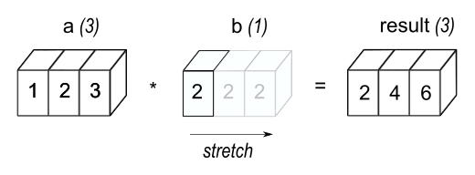
                        >>>                        a            =            np            .            assortment            ([            i.0            ,            2.0            ,            three.0            ])            >>>                        b            =            2.0            >>>                        a            *            b            array([ ii.,  4.,  vi.])

The result is equivalent to the previous instance where b was an array. We tin think of the scalar b being stretched during the arithmetics functioning into an array with the same shape as a . The new elements in b , as shown in Figure 1, are simply copies of the original scalar. The stretching analogy is only conceptual. NumPy is smart enough to use the original scalar value without actually making copies then that broadcasting operations are every bit retentiveness and computationally efficient every bit possible.

A scalar is broadcast to match the shape of the 1-d array it is being multiplied to.

Effigy ane ¶

In the simplest example of broadcasting, the scalar b is stretched to get an array of same shape as a so the shapes are compatible for element-by-element multiplication.

The lawmaking in the second example is more efficient than that in the first because broadcasting moves less memory around during the multiplication ( b is a scalar rather than an array).

General Broadcasting Rules¶

When operating on two arrays, NumPy compares their shapes element-wise. It starts with the trailing (i.e. rightmost) dimensions and works its way left. Two dimensions are compatible when

they are equal, or
1 of them is i

If these atmospheric condition are non met, a ValueError: operands could not exist broadcast together exception is thrown, indicating that the arrays have incompatible shapes. The size of the resulting array is the size that is not i along each axis of the inputs.

Arrays do not demand to have the same number of dimensions. For case, if yous accept a 256x256x3 array of RGB values, and yous want to calibration each color in the image by a different value, yous can multiply the prototype by a one-dimensional array with 3 values. Lining up the sizes of the trailing axes of these arrays according to the broadcast rules, shows that they are uniform:

                            Paradigm              (              three              d              array              ):              256              x              256              10              iii              Scale              (              1              d              array              ):              three              Result              (              3              d              array              ):              256              10              256              x              3

When either of the dimensions compared is i, the other is used. In other words, dimensions with size i are stretched or "copied" to lucifer the other.

In the following example, both the A and B arrays have axes with length one that are expanded to a larger size during the broadcast operation:

                            A              (              iv              d              assortment              ):              viii              ten              ane              ten              6              x              i              B              (              3              d              array              ):              7              ten              i              ten              5              Result              (              iv              d              assortment              ):              8              10              7              x              6              ten              5

Broadcastable arrays¶

A set of arrays is chosen "broadcastable" to the aforementioned shape if the above rules produce a valid result.

For instance, if a.shape is (5,1), b.shape is (1,vi), c.shape is (6,) and d.shape is () so that d is a scalar, and so a, b, c, and d are all broadcastable to dimension (5,half dozen); and

a acts similar a (five,half dozen) array where a[:,0] is broadcast to the other columns,
b acts like a (v,vi) array where b[0,:] is broadcast to the other rows,
c acts similar a (i,six) array and therefore like a (5,6) array where c[:] is broadcast to every row, and finally,
d acts like a (5,6) array where the single value is repeated.

Here are some more than examples:

                            A              (              ii              d              array              ):              5              x              iv              B              (              1              d              assortment              ):              1              Consequence              (              ii              d              array              ):              5              x              4              A              (              2              d              array              ):              5              x              4              B              (              1              d              array              ):              four              Outcome              (              2              d              assortment              ):              5              ten              4              A              (              three              d              array              ):              xv              x              3              10              5              B              (              3              d              assortment              ):              fifteen              x              1              x              five              Result              (              3              d              array              ):              xv              x              3              x              5              A              (              3              d              assortment              ):              15              x              three              x              v              B              (              ii              d              array              ):              3              ten              v              Result              (              iii              d              array              ):              15              ten              3              ten              v              A              (              3              d              array              ):              xv              ten              three              x              five              B              (              2              d              assortment              ):              3              x              1              Result              (              3              d              array              ):              fifteen              x              three              x              5

Here are examples of shapes that exercise non broadcast:

                            A              (              1              d              assortment              ):              three              B              (              1              d              assortment              ):              4              # abaft dimensions practice non match              A              (              two              d              array              ):              two              x              1              B              (              3              d              array              ):              8              x              4              x              three              # second from last dimensions mismatched

An example of broadcasting when a ane-d array is added to a 2-d assortment:

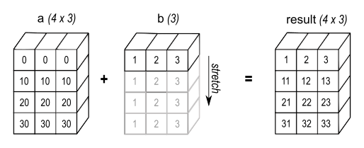
                            >>>                            a              =              assortment              ([[              0.0              ,              0.0              ,              0.0              ],              ...                            [              10.0              ,              10.0              ,              10.0              ],              ...                            [              twenty.0              ,              20.0              ,              twenty.0              ],              ...                            [              30.0              ,              thirty.0              ,              thirty.0              ]])              >>>                            b              =              array              ([              ane.0              ,              ii.0              ,              3.0              ])              >>>                            a              +              b              array([[  one.,   2.,   3.],                              [ xi.,  12.,  xiii.],                              [ 21.,  22.,  23.],                              [ 31.,  32.,  33.]])              >>>                            b              =              array              ([              1.0              ,              2.0              ,              3.0              ,              4.0              ])              >>>                            a              +              b              Traceback (about recent call terminal):              ValueError:              operands could non exist broadcast together with shapes (4,3) (4,)

As shown in Figure 2, b is added to each row of a . In Effigy 3, an exception is raised because of the incompatible shapes.

A 1-d array with shape (3) is strectched to match the 2-d array of shape (4, 3) it is being added to, and the result is a 2-d array of shape (4, 3).

Effigy 2 ¶

A one dimensional array added to a two dimensional array results in broadcasting if number of 1-d array elements matches the number of 2-d array columns.

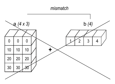
A huge cross over the 2-d array of shape (4, 3) and the 1-d array of shape (4) shows that they can not be broadcast due to mismatch of shapes and thus produce no result.

Figure 3 ¶

When the trailing dimensions of the arrays are unequal, broadcasting fails because it is impossible to align the values in the rows of the 1st array with the elements of the 2nd arrays for element-by-element add-on.

Dissemination provides a convenient way of taking the outer product (or any other outer performance) of two arrays. The post-obit example shows an outer add-on operation of two 1-d arrays:

                            >>>                            a              =              np              .              array              ([              0.0              ,              ten.0              ,              20.0              ,              30.0              ])              >>>                            b              =              np              .              array              ([              one.0              ,              2.0              ,              3.0              ])              >>>                            a              [:,              np              .              newaxis              ]              +              b              array([[  1.,   2.,   3.],                              [ 11.,  12.,  13.],                              [ 21.,  22.,  23.],                              [ 31.,  32.,  33.]])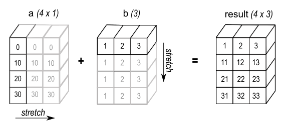

A 2-d array of shape (4, 1) and a 1-d array of shape (3) are stretched to match their shapes and produce a resultant array of shape (4, 3).

Effigy 4 ¶

In some cases, broadcasting stretches both arrays to form an output array larger than either of the initial arrays.

Here the newaxis alphabetize operator inserts a new centrality into a , making it a two-dimensional 4x1 array. Combining the 4x1 array with b , which has shape (iii,) , yields a 4x3 array.

A Practical Example: Vector Quantization¶

Broadcasting comes up quite oftentimes in existent world problems. A typical example occurs in the vector quantization (VQ) algorithm used in information theory, classification, and other related areas. The basic operation in VQ finds the closest point in a set of points, chosen codes in VQ jargon, to a given betoken, called the observation . In the very simple, two-dimensional case shown below, the values in observation draw the weight and elevation of an athlete to be classified. The codes represent dissimilar classes of athletes. ane Finding the closest point requires calculating the distance between observation and each of the codes. The shortest distance provides the best match. In this case, codes[0] is the closest class indicating that the athlete is probable a basketball thespian.

                            >>>                            from              numpy              import              array              ,              argmin              ,              sqrt              ,              sum              >>>                            ascertainment              =              array              ([              111.0              ,              188.0              ])              >>>                            codes              =              array              ([[              102.0              ,              203.0              ],              ...                            [              132.0              ,              193.0              ],              ...                            [              45.0              ,              155.0              ],              ...                            [              57.0              ,              173.0              ]])              >>>                            unequal              =              codes              -              observation              # the broadcast happens here              >>>                            dist              =              sqrt              (              sum              (              unequal              **              2              ,              centrality              =-              ane              ))              >>>                            argmin              (              dist              )              0

In this case, the observation array is stretched to match the shape of the codes assortment:

                            Observation              (              ane              d              array              ):              two              Codes              (              2              d              array              ):              4              x              two              Diff              (              2              d              assortment              ):              4              x              2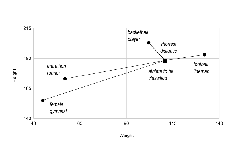

A height versus weight graph that shows data of a female gymnast, marathon runner, basketball player, football lineman and the athlete to be classified. Shortest distance is found between the basketball player and the athlete to be classified.

Figure 5 ¶

The basic performance of vector quantization calculates the distance between an object to be classified, the dark square, and multiple known codes, the gray circles. In this simple case, the codes stand for private classes. More complex cases use multiple codes per class.

Typically, a large number of observations , perhaps read from a database, are compared to a set up of codes . Consider this scenario:

                            Ascertainment              (              2              d              array              ):              10              x              three              Codes              (              2              d              array              ):              five              x              iii              Diff              (              3              d              array              ):              5              ten              10              x              3

The three-dimensional array, unequal , is a consequence of broadcasting, not a necessity for the adding. Large data sets will generate a big intermediate array that is computationally inefficient. Instead, if each ascertainment is calculated individually using a Python loop around the lawmaking in the two-dimensional example above, a much smaller array is used.

Dissemination is a powerful tool for writing brusk and commonly intuitive code that does its computations very efficiently in C. However, there are cases when broadcasting uses unnecessarily large amounts of memory for a detail algorithm. In these cases, it is better to write the algorithm's outer loop in Python. This may likewise produce more than readable code, as algorithms that apply dissemination tend to become more than difficult to translate as the number of dimensions in the circulate increases.

Footnotes

1: In this example, weight has more than impact on the altitude calculation than height because of the larger values. In exercise, it is of import to normalize the elevation and weight, often past their standard deviation across the data set, so that both accept equal influence on the distance calculation.